mAP 란?

mAP(mean Average Precision)는 자주 사용되고 Detection에서는 빠질 수 없는 지표이다.

하지만 이번에 회사에서 운영 부서에서 "Detection모델의 성능이 어떻게 되나요?" 라는 질문을 받았을때 쉽게 대답할 수 없었다. "저희 모델은 `mAP@0.5`가 0.89이상 나옵니다!" 하는데 어떻게 받아들일까?

이미 mAP 관련 글은 넘쳐나지만 누군가 보고 쉽게 이해할 수 있도록 정리를 해보려고 글을 작성해본다.

Precision과 Recall

Precision 과 Recall을 이해하기 위해서 우선 간단한 binary classification 모델의 10개 데이터에 대한 출력 결과를 살펴보자.
여기서는 class에 대한 모델의 class probability에 따라 정렬을 해둔 상태이다.

모델에 따라서 계산 방식이나 표현이 다르지만 confidence는 class에 대한 probabiliy로 생각하면 된다.

confidence	10%	20%	30%	40%	50%	60%	70%	80%	90%	100%
Ground Truth(정답)	0	1	1	1	0	1	0	1	0	1
Prediction (예측)	0	1	1	1	1	0	0	1	1	1

Precision

Precision(정밀도)는 얼마나 정밀한지 알아보는 지표이다. 즉, 모델이 정답이라고 결론을 내렸는데 그중에서 얼마만큼이 진짜 답인지를 나타내는것이다. 이는 아래처럼 계산할 수 있다. (confusion matrix에 대해서 잘 모른다면 Appendix 참고)

\[Precision = {TP \over {TP + FP}}\]

Recall

Recall은 한국말로 재현률이다. 즉 얼마나 상황이 재현되었냐가 궁금한 지표이다. 즉, 실제 True 중에서 얼마나 True라고 예측된걸까? 를 알아보는 지표이다.

\[Recall = {TP \over{TP + FN}}\]

</br>

자 이제 다시 돌아와서 위의 출력결과를 살펴보자.
우리는 모델의 출력을 그대로 믿지않고 모델의 confidence를 가지고 결론을 내리게 된다. 예를 들어서 70% 이상의 정확도를 보인 예측만 True로 인정한다면 아래의 표와 같이 그 아래의 확률에 대해서는 0으로 예측이 바뀌게 된다.

confidence	10%	20%	30%	40%	50%	60%	70%	80%	90%	100%
Ground Truth(정답)	0	1	1	1	0	1	0	1	0	1
Prediction (예측)	0	0	0	0	0	0	0	1	1	1

이때 TP는 2개, FP는 1개, FN는 4개다. 따라서 Precision과 Recall은 각각 0.67, 0.34이다.

문제는 여기서 발생하는데 설정한 모델 정확도 기준을 바꾼다면 성능도 바뀔 수 있다. 예를들어서 50% 이상의 정답을 True로 인정한다면 다음과 같이 된다.

confidence	10%	20%	30%	40%	50%	60%	70%	80%	90%	100%
Ground Truth(정답)	0	1	1	1	0	1	0	1	0	1
Prediction (예측)	0	0	0	0	1	0	1	1	0	1

이때 TP는 2개, FP는 2개, FN는 4개다. 따라서 Precision과 Recall은 각각 0.5, 0.34이다.

위의 결과와 비교해보면 단순히 threshold만 바꾸어줬는데 성능이 바뀐것이다. 이때 모든 threshold에서 성능을 알아보려면 Precision - Recall 그래프를 그려보면 된다.

우선 그래프를 그려보기 위해서 위의 각 threshold별 Precision과 Recall을 알아보자.

confidence	10%	20%	30%	40%	50%	60%	70%	80%	90%	100%
Precision	0.71	0.71	0.67	0.6	0.5	0.67	0.67	0.67	0.5	1
Recall	0.83	0.83	0.67	0.5	0.34	0.34	0.34	0.34	0.17	0.17

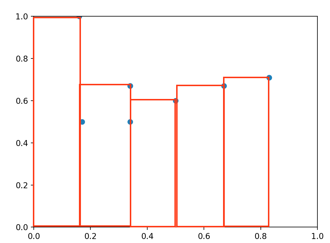
이를 그래프로 그려보면 다음과 같다.

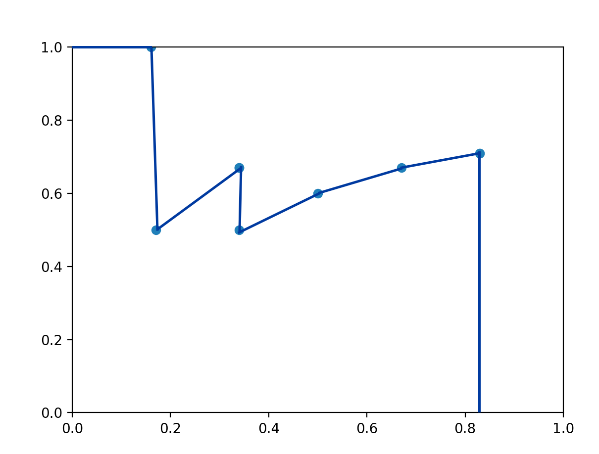
이때 파란선 아래쪽의 넓이를 구해보면 threshold와 상관없이 Precision, Recall 값에 의한 모델의 성능을 평가할 수 있다.

Detection?

이제 Detection의 예측 결과를 살펴보자.

Detection의 예측은 4개의 bounding box 정보와 class, confidence 값을 가지고 있다.
또한 예측한 bounding box가 맞을 수도 있고 물체는 없는데 위치할 수도 있다.
(아래 사진을 보면 초록색 GT box에 대비해서 정확한 예측(파란색 박스)도 있는 반면 예측이 잘못된 예측(노란색 점선 박스)도 발생한다.)

african-elephants-gfe56b7f74_640

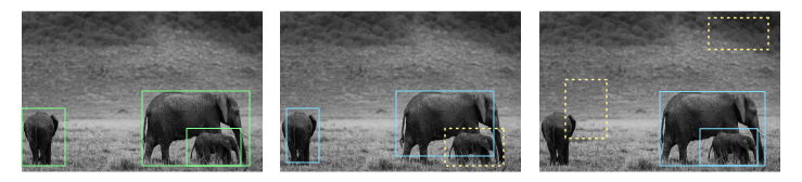
Pixabay로부터 입수된 Antony Trivet님의 이미지 입니다.

Detection 모델을 선택하기 위해서 Prediction bounding box와 GT bounding box 사이의 IOU, Prediction box와 GT bounding box의 유무에 따른 confusion matrix의 영향을 생각해야한다.

이때 confidence 값을 위의 그래프처럼 Precision-Recall 그래프로 만들어 아래 면적을 구하면 Prediction box와 GT bounding box의 유무에 따른 confusion matrix의 영향을 고려하며 모델을 선택할 수 있게된다.

좀더 자세하게 얘기하면 Prediction bounding box는 있는데 GT bounding box가 없는 경우(FP)나 Prediction bounding box는 없는데 GT bounding box가 있는 경우(FN)를 고려할 수 있다.

mAP 계산하기!

이제 이유를 알았으니 mAP를 구해보자.
mAP는 각 class에 대한 AP를 평균(mean)낸 값이다. 따라서 AP를 먼저 구해야한다.

이제 precision-recall 그래프를 그리면 된다는것을 알았기 때문에 모든 prediction에 대해서 출력값을 저장해주는 함수를 만든다.

  
class mAPCalculator():
    def __init__(self):
        # class ap_list shape : (n_classes,)
        self.ap_list = []

        # class confidence list. shape : (all_predictions, n_classes)
        self.all_confidences = None

        # TP, FP list. shape : (all_predictions,) if iou with G.T > threshold, and class is correct, 1 else 0.
        self.all_con_list = None

    def keep(self, cbboxes, cconfidences, target_id):
        '''
        NOTICE: calculate prediction is TP or FP and keep prediction information.
        :param cbboxes: (n_output_boxes, 4)
        :param cconfidences: (n_output_boxes, n_classes)
        :param target_id: {"boxes": boxes, "classes": classes} boxes : [n_target_boxes, [cell_x, cell_y, center_x center_y, w, h]],  classes: [n_target_boxes, category]
        :return:
        '''

        # Calculate which prediction is TP or FP
        cconfidences, con_list = self.calculate_confusion(cbboxes, cconfidences, target_id)

        # Stack confidences of predictions and is TP or FP
        self.all_confidences = cconfidences if self.all_confidences is None else np.concatenate([self.all_confidences, cconfidences], axis=0)
        self.all_con_list = con_list if self.all_con_list is None else np.concatenate([self.all_con_list, con_list], axis=0)

위의 함수를 통해서 데이터를 쌓으면 아래와 같은 구조로 데이터가 모이게 된다.

1. First, collect all box class, confidence, confusion information. 
(Just calculate precision recall for predictions on all Test Image.)
-----------------------------------------------------------------------------------------------
file        | class(argmax(confidences)) | confidence (:max(confidences)) | confusion
image01.png                 2                           0.88951                   1 (TP)
image02.png                 1                           0.93215                   1 (TP)
image01.png                 0                           0.85331                   0 (FP) 
image01.png                 0                           0.98245                   1 (TP)
image02.png                 2                           0.90457                   0 (FP)
.
.
.
-----------------------------------------------------------------------------------------------        
NOTICE: divide data by class and calculate confusion and merge them again.
NOTICE: when calculate confusion, if duplicated prediction occurred, set 0 confusion to next predictions.  

이때 confusion 정보는 GT bounding box와 예측 bounding box간의 IOU에 의해서 결정된다.

  
def calculate_iou_matrix(*coordinates):
    # Divide to each coordinates.
    x11, y11, x12, y12 = coordinates[:4]
    x21, y21, x22, y22 = coordinates[4:]

    # Choose edge of intersection.
    x_1 = np.maximum(x11, x21)  # intersection Left-Top x
    y_1 = np.maximum(y11, y21)  # intersection Left-Top y
    x_2 = np.minimum(x12, x22)  # intersection Right-Bottom x
    y_2 = np.minimum(y12, y22)  # intersection Right-Bottom y

    # Calculate intersection area.
    inter_area = np.maximum((x_2 - x_1), 0) * np.maximum((y_2 - y_1), 0)

    # Calculate iou.
    box1_area = (x12 - x11) * (y12 - y11)
    box2_area = (x22 - x21) * (y22 - y21)
    iou = inter_area / (box1_area + box2_area - inter_area + 0.001)

    return iou

def calculate_confusion(self, cbboxes, cconfidences, target):
        '''
        :param cbboxes: shape: (n_output_boxes, 4) ;[top_left_x, top_left_y, bottom_right_x, bottom_right_y]
        :param cconfidences: shape:(n_output_boxes, n_classes)
        :param target:  {"boxes": boxes, "classes": classes} boxes : [n_target_boxes, [cell_x, cell_y, center_x center_y, w, h]],  classes: [n_target_boxes, category]
        
        :return:
        cconfidences: valid prediction boxes. shape: (n_valid_predictions, 1); ex) 0.73456
        con_list: valid prediction boxes is correct or not. shape: (n_valid_predictions, 1); 1 is TP, 0 is FP.
        '''

        # Remove not valid boxes from two list.
        valid = np.max(cconfidences, axis=1) > 0

        # Remove zero confidence boxes.
        cconfidences = cconfidences[valid]
        cbboxes = cbboxes[valid]

        # Get classes.
        classes = np.argmax(cconfidences, axis=1)

        # TP, FP list.  # TP or FP : TP is 1, FP is 0
        con_list = np.zeros([len(cbboxes), 1], dtype=int)

        # Calculate AP for each class.
        for c in range(cfg.N_CLASSES):

            # Get each class boxes.
            output_boxes = cbboxes[np.where(classes == c)]

            # Target boxes flag. It is for prevent duplicated prediction.
            target_flag = np.zeros([len(np.where(np.array(target['classes']) == c)[0]), ], dtype=int)

            # target_boxes(G.T bounding boxes) on specific class.
            target_boxes = np.array(target['boxes'])[np.where(np.array(target['classes']) == c)]

            # Set TP, FP
            for tdx, t_box in enumerate(target_boxes):

                # Compare with 'output_boxes' and calculate IOU. next, set TP or FP
                for bdx, output_box in enumerate(output_boxes):

                    # each box shape : top_left_x, top_left_y, bottom_right_x, bottom_right_y
                    iou = calculate_iou_matrix(*output_box, *YOLO2CORNER(t_box))
                    # print(f'iou : {iou}')

                    # If TP, (generally, iou >= 0.5)
                    if iou > cfg.VALID_OUTPUT_THRESHOLD and target_flag[tdx] == 0:
                        # Set to TP.
                        con_list[np.where(classes == c)[0][bdx]] = [1]

                        # Set flag to 1. (when calculate AP, duplicated detection at last come to not correct prediction.)
                        target_flag[tdx] = 1

        return cconfidences, con_list

이 코드에서는 IOU threshold를 0.5로 잡았기 때문에 mAP를 구하는 경우 mAP@0.5로 표기할 수 있다. 논문을 보면 mAP@0.5:0.95 라는 표현을 볼 수 있는데 이는 mAP@0.5부터 mAP@0.95까지 0.05간격 값의 평균을 낸 값이다.

이제 데이터를 다 모았으면 confusion 값을 이용해서 Precision과 Recall 값을 계산한다.

AP 계산

AP는 하나의 class에 해당하는 Precision-Recall 그래프를 그려보면 된다.

|
|---------;
|         |
|         |
|         | 
|    A    |
|         ----------;
|         .    B    |
|         .         ----------;      
|         .         .    C       ...
|_______________________________________
|         |
T1        T2    ...

  
def calculate_AP(self, class_id, pre_rec):
        '''
        :param class_id: class id.
        :param pre_rec: shape : (n_prediction_boxes, 2); [precision, recall]
        :return: AP
        '''

        # Tn points.
        threshold = np.unique(pre_rec[:, 1])

        # Sum of below region.
        val_AP = 0

        for tdx, th in enumerate(threshold):
            # Calculate portion(A) divided by threshold.
            if tdx == 0:
                val_AP += np.max(pre_rec[:, 0][pre_rec[:, 1] <= th]) * th

            else:
                # Calculate portion(B, ...) divided by threshold.
                val_AP += np.max(pre_rec[:, 0][(threshold[tdx - 1] < pre_rec[:, 1]) & (pre_rec[:, 1] <= th)]) * (th - threshold[tdx - 1])

        return val_AP

여기서 작성한 코드에서는 유니크한 Recall값에 대해서만 대략적인 넓이를 구하고 있다. 일반적으로는 11 point interpolation, All point interpolation 을 사용하게 된다. (Apeendix 참조)

각 class에 대해 AP 구하고 평균 구하기

이제 AP를 구하는 코드를 작성했으니 앞서 데이터를 쌓아두었던 데이터를 confidence 순으로 정렬한다. 그리고 각 class 별로 테이블을 분리하여 각 class별 AP를 계산해준다.

2. Sort by descending confidence.
(Don't need to know about which predictions are placed on which image because just calculate precision recall for all predictions.)
-------------------------------------------------------------------------------
class(argmax(confidences)) | confidence (:max(confidences)) | confusion
0                           0.98245                   1 (TP)
1                           0.93215    |              1 (TP)
2                           0.90457    |              0 (FP) 
2                           0.88951    V              1 (TP)
0                           0.85331                   0 (FP)
.
.
.
-------------------------------------------------------------------------------            

3. divide matrix by class and calculate precision and recall.
-------------------------------------------------------------------------------

=================================class0================================
class(argmax(confidences)) | confidence (:max(confidences)) | confusion
0                           0.98245                   1 (TP)
0                           0.85331                   0 (FP)
.
.
.
=================================class1================================
class(argmax(confidences)) | confidence (:max(confidences)) | confusion
1                           0.93215                   1 (TP)
.
.
.
=================================class2================================
class(argmax(confidences)) | confidence (:max(confidences)) | confusion
2                           0.90457                   0 (FP) 
2                           0.88951                   1 (TP)
.
.
.
-------------------------------------------------------------------------------

4. Calculate mAP or just show AP of each class.   

  
def calculate(self, plot=True, mean=True):
        '''
        :param plot:
        :param mean:
        :return:
        '''

        # sort all confidence.
        classes = np.argmax(self.all_confidences, axis=1)
        all_confidences = np.max(self.all_confidences, axis=1)

        # Get sorted index by  descending class confidence
        sorted_index = np.argsort(all_confidences, axis=0)[::-1]

        # Sort confidence by descending order.
        all_confidences = np.squeeze(all_confidences[sorted_index])
        if cfg.N_CLASSES == 1: all_confidences = np.expand_dims(all_confidences, axis=-1)
        all_con_list = np.squeeze(self.all_con_list[sorted_index])

        for c in range(cfg.N_CLASSES):
            # Using 'all_predict', 'output_confidences' and 'con_type', calculate AP for each class.

            # choose specific class.
            one_class_confidence = all_confidences[np.where(classes == c)]
            one_class_con_list = all_con_list[np.where(classes == c)]

            # calculate TP +FN, all box predictions for in each class.
            all_predict = sum(one_class_con_list)

            # Precision and recall.
            pre_rec = np.zeros([len(one_class_confidence), 2])

            # Calculate precision and recall.
            for row in range(len(one_class_confidence)):
                precision = sum(one_class_con_list[:row + 1]) / (row + 1)
                recall = sum(one_class_con_list[:row + 1]) / all_predict

                # Update pre_rec
                pre_rec[row] = [precision, recall]

            # Add to ap_list (AP for each class.) shape:[C]
            ap = self.calculate_AP(c, pre_rec, plot)
            print(f'AP_{cfg.CLASS_NAME[c]} : {ap}')
            self.ap_list.append(ap)

        return np.mean(self.ap_list) if mean else self.ap_list

이렇게 정리하고 보니 더 설명하기 애매해진 것 같다.

그냥 사용 예시를 남기고 마무리 한다.

  
cal_mAP = mAPCalculator()

for iteration, (img, target) in enumerate(test_loader):
    # For calculate FPS.
    before = time.time()

    inputs = torch.stack(img)
    outputs = model(inputs)

    # TEST: without NMS
    for id, output in enumerate(outputs):
        img = np.transpose(inputs[id].detach().numpy(), [1, 2, 0])

        # output boxes after NMS.
        # cbboxes shape : [n_output_boxes, 4]
        # cconfidences shape : [n_output_boxes, n_classes]
        cbboxes, cconfidences = non_maximum_suppression(output)

        # Keep predict boxes information for calculate mAP.
        cal_mAP.keep(cbboxes, cconfidences, target[id])

# Calculate mAP.
result = cal_mAP.calculate(plot=True, mean=True)
print(f'mAP : {result}')

위의 코드는 scratch로 전체적인 detection의 구조를 설명하고자 만들었던 프로젝트의 일부 코드이다. non_maximum_suppression 코드나 기타 내용을 보고 싶으면 레포를 살펴보면 좋을것 같다.

Appendix

Confusion matrix (2 x 2)

-	-	실제 정답
-	-	1	0
모델의 출력	1	True Positive	False Positive
	0	False Negative	True Negative

위의 그래프에서 볼 수 있듯, 위의 지표들의 의미는 다음과 같다.

TP(True Positive) : 맞는 긍정이다 (모델이 맞다(Positive, 1)고 했더니 진짜더라(True))
FP(False Positive) : 틀린 긍정이다 (모델이 맞다(Positive, 1)고 했더니 알고보니 아니더라(False))
TN(True Negative): 맞는 부정이다 (모델이 아니다(Negative, 0)고 했더니 진짜더라(True))
FN(False Negative): 틀린 부정이다 (모델이 아니다(Negative, 0)고 했더니 알고보니 아니더라(False))

11 point interpolation

11 point interpolation은 말그대로 Precision-Recall 그래프에서 Recall값을 11단계로 나누고 그 점들의 Precision 값을 interpolate해서 아래 면적을 구한다.

계산 수식은 다음과 같다.

\[\mathbf{AP} = {1\over11} \sum_{r \in \left\{0, 0.1,...,1\right\}} \rho_{\mathbf{interp}(r)}\] \[\rho_{\mathbf{interp}(r)} = \max_{\tilde{r}:\tilde{r} \ge r} \rho(\tilde{r})\]

수식을 살펴보면 $r$이 0일때 0보다 큰 Recall 값중에서 Precision 값이 max인 값을 선택하고 0.1일때는 0.1보다 큰 Recall값 중에서 Precision값이 max인 값을 선택하는 식으로 11개의 point에 대해 계산을 하면 된다.

Interpolating all points

11 point 방식과 다르게 모든 지점에 대해서 interpolating을 수행하게 된다.

\[\sum_{n=0}(r_{n+1} - r_{n}) \rho_{\mathbf{interp}(r)} (r_{n+1})\] \[\rho_{\mathbf{interp}(r)} (r_{n+1}) = \max_{\tilde{r}:\tilde{r} \ge r_{n+1}} \rho(\tilde{r})\]

수식을 살펴보면 앞서 11 point 방식에서는 다음 $r$이 고정되는것과는 다르게 다음 $r_{n+1}$을 $r_{n}$으로 선택해주면 된다.

Reference

[1] rafaelpadilla/Object-Detection-Metrics#11-point-interpolation
[2] Pascal VOC challenge
[3] Pascal VOC challenge paper
[4] https://www.waytoliah.com/1491
[5] https://ctkim.tistory.com/79
[6] https://junha1125.tistory.com/51
[7] https://jonathan-hui.medium.com/map-mean-average-precision-for-object-detection-45c121a31173

mAP 쉽게 살펴보기